
Getting Your Data Ready for a Pivot Table

Get your data Pivot Table ready with Power Query. In this tutorial you will see how to use Power Query to unpivot, pivot and transpose your data. You will not only go through exercises, which you can download, so that you can follow along. You will also understand why and how to unpivot, transpose and Pivot your data.
Unpivot, Pivot and Transpose
When it comes to Unpivot, Pivot and Tranposing data it can be difficult to know which one you should go for. Truth is that you use a combination of all three to get the job done. You might start of with transposing data, then clean the data a bit. Then you would unpivot necessary columns, a little more tidying. Finally, pivoting columns seals the deal.
Power Query for Newbies Free Tutorial
Alright then, let's go through the meaty session so you can see how to use a combination of unpivot, pivot and transpose to change the following data. (Download here).

How can Power Query help?
The above data is a spreadsheet that you will commonly see. The months are running across the top as row headers. The areas are sort of like sub-headings with the data.
Our challenge is not only to clean up this data so that it is reading to be used to create a Pivot Table. It is also to create a system, a filter system if you will, that will automatically update the Pivot Table when the data is updated. This is where Power Query comes in. We can use Power Query to create a step by step process that automatically filters data into a Pivot Table. This will save you ever having to clean up this data again.
Exercise - Getting data ready for a Pivot Table
OK let's take this step-by-step, first select the data.
Now click on Data - From Table/Range.

Untick My table has headers.
(
We don't want to promote the column headers yet, this will give us greater flexibility in working with the data as we import the data into Power Query and hence get it ready for analysis with a Pivot Table.)

Click OK.
First thing we will do is to transpose the data. Click Transform - Transpose.

(Transpose effectively swaps the rows to columns, in effect what were row headers have now become column headers. We need to do this as we need all the columns that contain the areas, these would be columns 1, 5, 9, 13.)
Click anywhere inside the grid in Power Query and select all by pressing Ctrl & A.
Now click Fill - Down.

Have a look at column1 and the subsequent area columns. They have been filled down. We need to do this so that we can apply an area to each of the rows. Now it's time to promote the first row to column headers.
Click Use First Row as Headers.

(If you look at the column headers you will see that they now look like:)

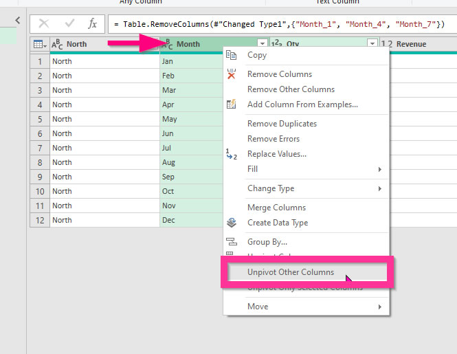
Now remove the Month_1, Month_4 and Month_7 columns.
(You can use the Ctrl key to select them and press delete to remove them.)

(Note that the Month column should still be there, you shouldn't delete that. But we don't need to duplicate month columns).
Next we need to unpivot all the columns except the Month column. Unpivoting all the other columns will keep the month column as it is however all the other columns will be unpivotted so that the column headers will become rows.
Right-click the Month column and choose Unpivot other columns.
When you now look at the data you can see that the month column has the month repeated as necessary, whereas the column headers of areas, Qty and Revenue have been converted into rows. You can also see that the Qty and Revenue rows have a number added to the end. Qty_2 or Revenue_3. This is because these rows where columns, and you can't have 2 columns with the same column header name.

Next we need to create the Area column. We're going to use a Conditional Column to accomplish this. Basically, we will check to see if Attribute and value are the same. If so, then we will write that value in the new area column.
Before we create the conditional column, however, we will change the data type for Value to Text so that the comparison can be done easily.
Select the data type button on the left of the Value column and change to Text.

Now, click Add Column from the ribbon,

Enter the following details:
- New column name: Area
- Column Name: Attribute
- Operator: Equals
- Value: Value
(Choose Select a column)

- Output: Choose Select a column as above then Value.

Click OK.
Now you should see the new area column with the areas that match the appropriate qty and revenue.

With the Area column selected click Transform - Fill - Down. (As we did before).
The next thing that we need to do is to filter out the North, South, East and West areas from the Attribute column.
Click the filter drop down menu of the attribute column and untick North, South, East and West.

Click OK.
Next, we need to split the attribute column using the underscore as a delimiter. In this way when we Pivot the data back to column headers we don't get duplicate column headers.
Ensure that the attribute column is selected then click Split column from the Transform tab and choose from delimiter.

In the next box see that the underscore has automatically been selected as the delimiter. This is exactly what we want.

Click OK.
Now, let's delete the Attribute.2 column that was created when we split the column be delimiter. Highlight the Attribute.2 column and press delete on the keyboard.

Click Attribute.1 then click Pivot Column from the Transform tab.

From the Values drop-down list choose Value, then expand the Advanced Options and select Don't Aggregate.

Click OK.
Your data is almost ready to go the last thing to do is to change the data types of revenue to currency and qty to whole number and area to text.

Next double click on the Table1 name and change it to SalesData.

Finally, we will load the data back into Excel.
Click Home - Close & Load.

Now the data is loaded into a Pivot Table. Now if you're followed this so far I don't need to tell you how to make a Pivot Table. But you now know how to make data ready for a Pivot Table.
Conclusion
Not every spreadsheet is the same, there will always be different solutions to getting your data pivot table ready. However, making good use of Unpivot, Pivot and Transpose will help you bucketloads in cleaning up your data, restructuring your data so that you can actually create a Pivot Table.
Extra Training
Pre-recorded tutorials are one thing, but an instructor led training course is something else. Check out what's covered on our Intermediate and Advanced Excel 365 Training Courses.
Should you or any member or your organisation want additional help then please either give us a call or fill out an enquiry form. We'd love to hear from you.